- Wed 10 January 2018
- Article
- Glen Berseth
- #RL, #DeepLearning
comments: true
Intro
In recent years there has been an explosion in Deep Reinforcement learning research resulting in the creation of many different RL algorithms that work with deep networks. In DeepRL and RL, in general, the goal is to optimize a policy \(\pi(a|s,\theta)\) with parameters \(\theta\) with respect to the future discounted reward.
It can be difficult to keep track of the many algorithms, let alone their properties, and when it is best to use which one.
In this post, I make an effort to organize several RL methods into a few groups. This organization helps clear up some misconceptions of different algorithms and demystifies what these properties mean, for example, on-policy vs off-policy.
Algorithms and Properties
Here a table of popular RL algorithms is given.
| Name | on/off policy | action space support | exploration method |
|---|---|---|---|
| TRPO | on-policy | discrete and continuous | e-greedy and Gaussian noise |
| DDPG | off-policy | continuous only | Ornstein–Uhlenbeck process |
| A3C | on-policy | discrete and continuous | e-greedy and Gaussian noise |
| CACLA | on-policy | continuous | e-greedy and Gaussian noise |
| DQN | off-policy | discrete | e-greedy |
| A2C | on-policy | discrete and continuous | e-greedy and Gaussian noise |
| Q-Prop | on-policy | discrete and continuous | e-greedy and Gaussian noise |
| PPO | on-policy | discrete and continuous | e-greedy and Gaussian noise |
| CEM | on-policy | discrete and continuous | e-greedy and Gaussian noise |
Properties
Exploration Method:
- e-greedy: Is primarily used for discrete action domains. The main idea being that a random action should be chosen with a non-zero probability.
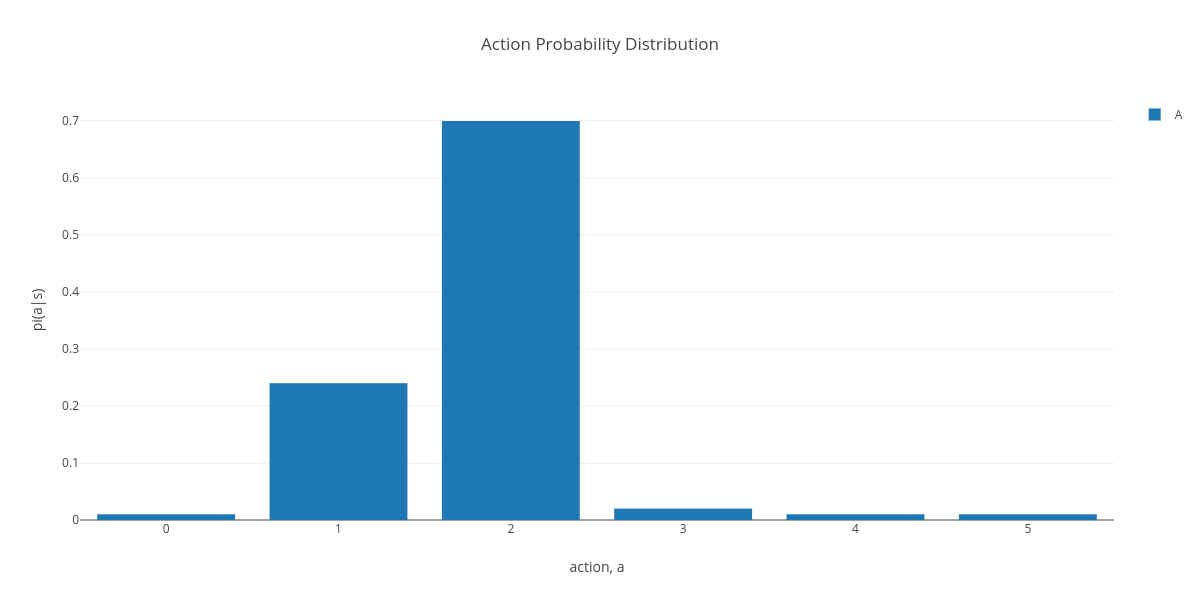 Original action selection probability
|
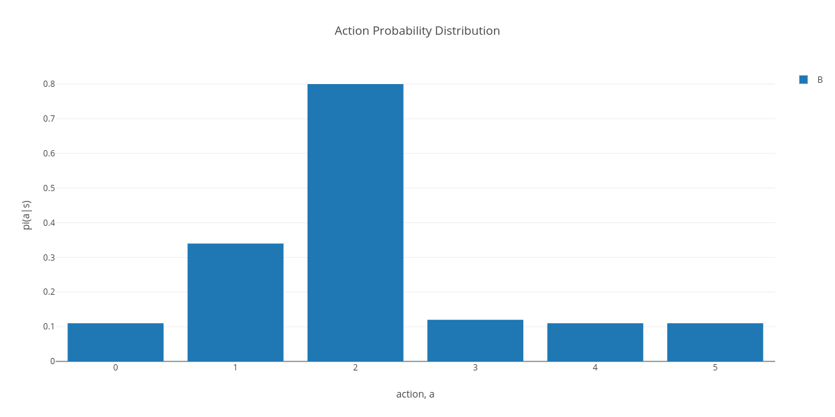
with epsilon greedy |
- Gaussian: Is typically for continuous action domains and one of a few methods used. Many methods using the neural network to model the mean of a number of Gaussian distributions that may have a fixed variance.
- Ornstein–Uhlenbeck This is a different kind of exploration noise that is based on "the velocity of a massive Brownian particle under the influence of friction". Often used for Q-learning with DDPG.
One property of RL algorithms I still rack my brain is on-policy vs off-policy. The line between these two very fuzzy. While it is known that any method that uses an action-valued function is off policy, some methods that claim to be on-policy are used in ways that seem very off-policy. In some papers, the amount of data collected before performing training updates is in the 100,000s, far more than anything I have ever used for off-policy learning. It has also been shown that keeping around data from the last few data collection cycles is beneficial. We also seem to gloss over the fact that we do not train the policy and value function to convergence between data collection cycles. Therefore, in practice, we are always using an off-policy critic.
Learning algorithms
Continuous Actor-Critic Learning Automaton (CACLA)
CACLA can be thought of as a simpler policy learning algorithm that was developed before some of the new formal mathematical methods. A critic (value function) and policy are learned at the same time (aka actor-critic method). CACLA uses the critic as a score function to decide from which actions the policy should learn. In this case, it is used as an indicator function, an action that performs better than the current estimate of the policies future discounted reward is given to the policy for training. The policy uses MSE loss to fit the policy network to these better than expected actions.
Pros:
- CACLA seems to work very well with neural networks. Being able to use a simple MSE loss for the policy makes SGD very stable.
Cons:
- Cannot adjust the amount of exploration the policy should perform.
- The original method only uses single-step returns to determine if the reward for action is above average.
Asynchronous Actor-Critic (A3C)
A3C can be thought of as a modification of CACLA in at least two ways. The MSE loss is traded with a log-likelihood loss, and the score function is exchanged for a multi-step return estimation. Switching to a log-likelihood loss allows us to model the distribution of action better, including the policy variance. In the case of continuous actions, the policy is modeled as a vector of Gaussian distributions. This allows for a better trade-off between the bias of the value function and the variance in Monte-Carlo samples from the simulation allows us to include a loss for the variance in the policy. Now we can update the amount of exploration we think the policy should be performing in an on-policy state-dependent manner.
Pros:
- Using the on-policy method with log-likelihood loss allows the exploration to be learned.
- The method can be parallelized well.
Cons:
- In practice, stable exploration is still a challenge. An Entropy term is added to the loss to help increase exploration.
- The policy mean can still change dramatically between training updates, making it challenging to converge on a good policy.
Deep Deterministic Policy Gradient (DDPG)
DDPG is a slightly different framework, more like DQN. Instead of using a score function to push the policy in the direction of actions with higher reward using the stochastic policy gradient, instead, an action-valued Q-function is used. This action-valued function \(q(s,a)\) can be used to compute the direction to change the current action in order to increase the overall future discounted reward. Simply, the method maximizes \(q(s,\pi(a|s))\). However, this method does not account for how exploration should be performed. Approximating a Q-function is done off-policy, allowing the Q-function to learn the value of taking actions in states the policy might not explore and in doing so, better estimate the value over all actions. This property should theoretically allow for the learning of a Q-function that encodes the best action to take in any state. In practice this model learns estimates over the current policy mean in order to improve the policy.
Pros:
- It can work very well for high dimensional continuous action problems.
- Learns an action-valued function instead of a state-valued function.
Cons:
- Does not explicitly provide a formalism for the exploration to be used.
- Needs a target network to increase stability while learning an action-valued function.
- The policy is only as good as the Q-function is accurate...
Trust Region Policy Optimization (TRPO)
TRPO is an algorithm with some good theoretical properties. Stochastic policy optimization can be challenging because the policy distribution can change quickly after network updates. These quick changes, in combination with the properties of deep neural networks, in particular, that deep nets like to receive small gradients, make learning challenging. When the stochasticity grows, so do the gradients; when the gradients grow, so does the stochasticity of the policy. TRPO uses conjugate gradient descent with a line search to optimize the policy parameters \(\theta\) with respect to a constraint on the KL divergence. The use of a KL constraint assists in keeping the policy's stochastic distribution from changing to much between updates.
Pros:
- TRPO can work very well and is known even to exhibit monotonic policy improvements.
Cons:
- Challenging to use TRPO for things like recurrent neural networks.
- Lots of memory is needed to compute the Fisher vector product (AKA gradient vector product) of the parameters \(\theta\)
- Not easily parallelizable.
Generalize Advantage Estimation (GAE)
While not an RL algorithm, GAE is used to reduce the variance in the advantage estimates for the policy. TRPO uses a KL divergence penalty to reduce the amount the policy distribution can shift between updates. However, there can still be a significant variance in the advantage estimate.

Here we can see a set of states labeled with their future discounted reward;advantage (from samples);baseline. The True policy gradient is visualized with the ellipses. One of the challenges with estimating the Advantage is that it is based on the future discounted reward. The agent could have randomly found some suitable reward for a few timesteps and then wandered into a very low reward area of the state space. The low average reards will result in a low overall future discounted reward and a high Advantage for the states the agent explored in the high reward area. This advantage is good, but for practical reasons having widely different advantage values can lead to large and noisy gradients.
GAE reduces the variance by mixing the advantage estimates from just the data with estimates computed from the returns using the value function (baseline).
Proximal Policy Optimization (PPO)
PPO was born from work that was done to combat the weaknesses of TRPO while keeping monotonic behaviour. PPO uses stochastic gradient descent instead of conjugate gradient descent to optimize the policy parameters. Instead of a hard constraint on the KL divergence, a soft constraint is used. This constraint is implemented in the form of a boundary violation penalty or a clipping term (the official version). PPO has been shown to have close to or better performance than TRPO.
Pros:
- Parallelizable.
- Does not use as much memory as TRPO
Cons:
- KL can still change significantly between updates. Some network-tuning could be necessary
Q-Prop (Q-Prop)
It would be really nice if we could combine the good parts of off-policy learning with those of on-policy learning. Q-Prop is one of a few works in this area. The goal is to combine the gradients from DDPG with unbiased on-policy data. Methods like DDPG can never be extremely accurate because the gradients passed to the actor come from an imperfect deep network with its own error. To get around this inaccuracy, it is better to use data samples to reduce this error directly. Q-Prop does this by using an additional estimate of the advantage function (as the Q-function from DDPG) as a control variate to reduce the advantage variance from GAE.
This estimate works to reduce the advantage variance further, However, it might not be so clear that this method is an imrovement.
Discussion
There has been a considerable amount of RL research that shows RL has promise and can find high-value solutions. However, RL still suffers from a tenancy to get trapped in local minima. Some believe this is related to the basic models we use for policy distributions. In this area, some people have used parameter space noise exploration instead of action space (Parameter Space Noise for Exploration,Noisy Networks for Exploration). Others are doing work on better frameworks to exploit the data better. Still, more work using Stochastic Value Gradients learns a model to optimize the stochastic bellman equation. A Distributional Perspective on Reinforcement Learning focuses on learning an approximate value distribution. A similar method has been applied to DDPG as well Distributed Distributional Deterministic Policy Gradients
There are still many more RL algorithms than the ones mentioned here. These are the ones that are popular, and I am more familiar with. This post has followed a road map of how RL research has progressed and why. There are many other aspects to consider when using an RL algorithm, such as: how difficult is the problem to be solved, how many dimensions is the action space, does the state include images, etc. If you are interested in using an RL algorithm, I suggest picking one off this list and possibly research some of the related papers that may have made small modifications to the algorithm. Also, checking for papers/projects that solved a problem similar to what you are working on is a good start.